Derivative Analysis & Quotient Rule
This lesson focuses on reading derivative graphs to determine where a function increases, decreases, and attains its local extrema. We also develop the Quotient Rule — a formula for differentiating a fraction — which arises whenever one changing quantity is divided by another.
When engineers design structures, they must determine where a curve rises, falls, and attains its peaks and valleys — precisely the information that derivatives encode. The quotient rule arises whenever one computes a rate such as “miles per gallon” or “points per game” — any situation involving the division of one changing quantity by another.
Topics Covered
- Polynomial graphing: the snaking method (continued practice)
- Multiplicity at roots: even power = bounce, odd power = cross
- Reading the derivative graph \(f'(x)\) to understand \(f(x)\)
- Identifying maxima, minima, and stationary points from sign changes in \(f'(x)\)
- Differentiating fractions by rewriting as powers of \(x\)
- The Quotient Rule: \(\displaystyle\frac{d}{dx}\!\left(\frac{P}{Q}\right) = \frac{Q \cdot dP - P \cdot dQ}{Q^2}\)
Lecture Video
Key Frames from the Lecture
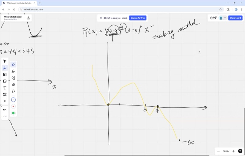
Polynomial Graphing: The Snaking Method
To use the snaking method, one must first write the polynomial in factored form. For example:
\[x^3 - 4x = x(x-2)(x+2)\]
The factors determine the roots (where the graph touches or crosses the x-axis). Once the roots are known, one can snake through them.
The snaking method is a quick way to sketch a polynomial:
- Find the roots from the factored form.
- Mark them on the x-axis.
- Check the leading term to know if the graph starts high or low on the right.
- Snake through the roots — crossing at odd-multiplicity roots, bouncing at even-multiplicity roots.
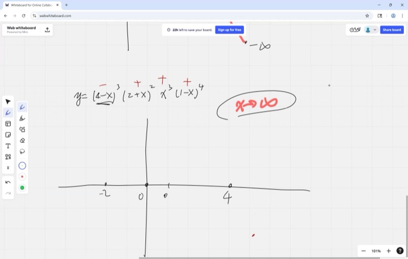
Multiplicity and Behavior at Roots
The power (multiplicity) of each factor tells you what happens at that root:
| Factor | Multiplicity | Behavior at root |
|---|---|---|
| \((x - r)^1\) | 1 (odd) | Graph crosses the x-axis |
| \((x - r)^2\) | 2 (even) | Graph bounces off the x-axis |
| \((x - r)^3\) | 3 (odd) | Graph crosses with a flat S-shape |
| \((x - r)^4\) | 4 (even) | Graph bounces (flatter than square) |
Odd power = cross. Even power = bounce.
Why? Because \((x - r)^{\text{even}}\) is always \(\geq 0\) — a square (or fourth power, etc.) can’t be negative. So the graph can’t go through to the other side. But \((x - r)^{\text{odd}}\) changes sign, so the graph must cross.
Explore multiplicity — drag the sliders to change the powers:
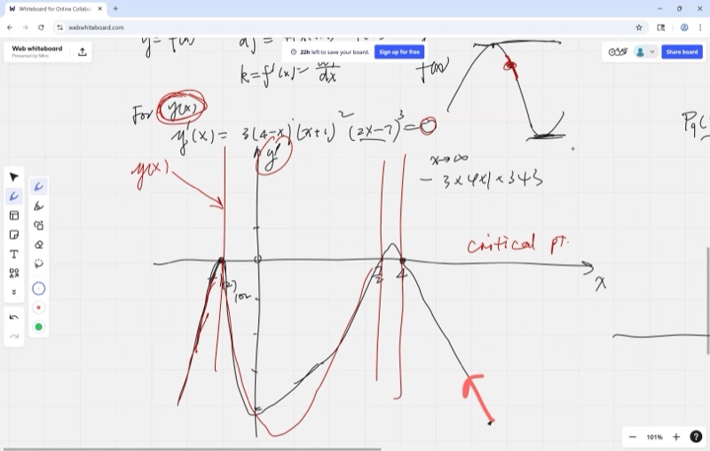
Critical Points and Reading the Derivative Graph
The derivative \(f'(x)\) gives the slope of \(f(x)\) at every point. If \(f'(x) > 0\), the original function is increasing. If \(f'(x) < 0\), it is decreasing. If \(f'(x) = 0\), the function is momentarily flat — a critical point.
The derivative graph \(f'(x)\) serves as a complete summary of the behavior of the original function \(f(x)\):
| What \(f'(x)\) does | What \(f(x)\) does |
|---|---|
| \(f'(x) > 0\) (above x-axis) | \(f(x)\) is increasing (going up) |
| \(f'(x) < 0\) (below x-axis) | \(f(x)\) is decreasing (going down) |
| \(f'(x) = 0\) (crosses x-axis) | \(f(x)\) has a critical point (flat) |
Identifying Maxima, Minima, and Stationary Points
A critical point (where \(f'(x) = 0\)) can be one of three types. One determines the classification by examining how \(f'(x)\) changes sign:
Examine the sign of the derivative immediately before and after a critical point. The sign change (or lack thereof) determines exactly what type of critical point is present.
| Sign change in \(f'(x)\) | Type of critical point |
|---|---|
| \(+ \to -\) (positive then negative) | Local maximum |
| \(- \to +\) (negative then positive) | Local minimum |
| No sign change (\(+ \to +\) or \(- \to -\)) | Stationary inflection point |
- Maximum: The function was increasing (\(f' > 0\)), reaches a peak, then begins decreasing (\(f' < 0\)).
- Minimum: The function was decreasing (\(f' < 0\)), reaches a trough, then begins increasing (\(f' > 0\)).
- Stationary inflection: The derivative momentarily equals zero, but the function continues in the same direction — intuitively, this corresponds to a brief flattening along the curve.
Explore: see \(f(x)\) and \(f'(x)\) side by side:
Observe that \(f'(x) = 0\) at \(x = -1\) and \(x = 1\) — precisely where \(f(x)\) attains its local maximum and minimum.
Animated: Sign chart showing how f’(x) positive/negative maps to f(x) increasing/decreasing
Derivative Sign Chart for f(x) = x³ - 3x
Differentiating Fractions: Rewriting as Powers
Recall that \(\dfrac{1}{x^n} = x^{-n}\). This identity allows us to convert fractions into power functions that can be differentiated using the power rule.
Before developing the quotient rule, we note a simpler technique that applies when the denominator is a power of \(x\): rewrite the fraction as a sum of powers.
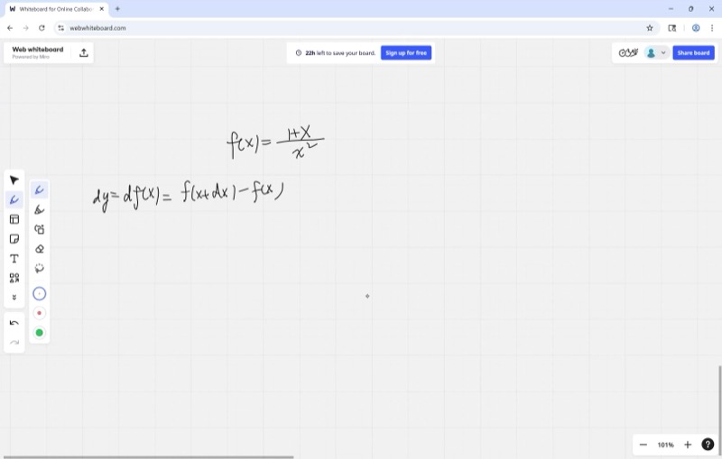
Example: Differentiate \(\dfrac{1 + x}{x^2}\).
Step 1: Split the fraction:
\[\frac{1 + x}{x^2} = \frac{1}{x^2} + \frac{x}{x^2} = x^{-2} + x^{-1}\]
Step 2: Apply the power rule to each term:
\[\frac{d}{dx}\left(x^{-2} + x^{-1}\right) = -2x^{-3} + (-1)x^{-2} = -\frac{2}{x^3} - \frac{1}{x^2}\]
This approach avoids the quotient rule entirely and should be used whenever applicable.
The Quotient Rule
The quotient rule is built on the product rule. Recall: if \(y = P \cdot Q\), then
\[\frac{dy}{dx} = P \cdot \frac{dQ}{dx} + Q \cdot \frac{dP}{dx}\]
The quotient rule handles \(P/Q\) instead of \(P \cdot Q\).
Given a fraction \(\dfrac{P}{Q}\) where both \(P\) and \(Q\) are functions of \(x\), the quotient rule states:
To differentiate a fraction, use “bottom times derivative of top, minus top times derivative of bottom, all over bottom squared.”
\[\frac{d}{dx}\!\left(\frac{P}{Q}\right) = \frac{Q \cdot \dfrac{dP}{dx} \;-\; P \cdot \dfrac{dQ}{dx}}{Q^2}\]
Start with \(y = \dfrac{P}{Q}\). When \(x\) changes by a tiny amount \(dx\):
- \(P\) changes to \(P + dP\)
- \(Q\) changes to \(Q + dQ\)
So the new value is \(\dfrac{P + dP}{Q + dQ}\). The change in \(y\) is:
\[dy = \frac{P + dP}{Q + dQ} - \frac{P}{Q}\]
Put both fractions over a common denominator \(Q(Q + dQ)\):
\[dy = \frac{Q(P + dP) - P(Q + dQ)}{Q(Q + dQ)} = \frac{Q \cdot dP - P \cdot dQ}{Q(Q + dQ)}\]
Since \(dQ\) is infinitesimally small, \(Q + dQ \approx Q\), so:
\[\frac{dy}{dx} = \frac{Q \cdot \dfrac{dP}{dx} - P \cdot \dfrac{dQ}{dx}}{Q^2}\]
Animated: Quotient Rule visualized as rectangle areas
Quotient Rule: Q·P' − P·Q' over Q²
Example: Differentiate \(\dfrac{x^2 + 1}{x - 3}\).
Let \(P = x^2 + 1\) and \(Q = x - 3\). Then \(\dfrac{dP}{dx} = 2x\) and \(\dfrac{dQ}{dx} = 1\).
\[\frac{d}{dx}\!\left(\frac{x^2+1}{x-3}\right) = \frac{(x-3)(2x) - (x^2+1)(1)}{(x-3)^2} = \frac{2x^2 - 6x - x^2 - 1}{(x-3)^2} = \frac{x^2 - 6x - 1}{(x-3)^2}\]
Explore the function and its derivative:
Cheat Sheet
| Concept | Key Formula / Rule |
|---|---|
| Multiplicity at roots | Odd power = cross, even power = bounce |
| \(f'(x) > 0\) | \(f(x)\) is increasing |
| \(f'(x) < 0\) | \(f(x)\) is decreasing |
| \(f'(x) = 0\), sign \(+ \to -\) | Local maximum |
| \(f'(x) = 0\), sign \(- \to +\) | Local minimum |
| \(f'(x) = 0\), no sign change | Stationary inflection point |
| Rewriting fractions | \(\dfrac{1+x}{x^2} = x^{-2} + x^{-1}\), then use power rule |
| Quotient Rule | \(\dfrac{d}{dx}\!\left(\dfrac{P}{Q}\right) = \dfrac{Q \cdot dP - P \cdot dQ}{Q^2}\) |