Euler’s Formula & Functional Equations
This lesson derives Euler’s formula, one of the most celebrated identities in mathematics. It connects three seemingly unrelated domains — exponentials, trigonometry, and imaginary numbers — into a single identity. We arrive at it by investigating the functional equation “what type of function converts addition into multiplication?” The answer leads directly to \(e^{i\theta} = \cos\theta + i\sin\theta\), with logarithms serving as the bridge between multiplicative and additive structures.
Euler’s formula connects exponentials, trigonometry, and complex numbers in a single identity. Functional equations allow one to deduce what a function must be from its algebraic properties alone:
- Electrical engineering: AC circuits use \(e^{i\omega t}\) to represent oscillating voltages and currents — Euler’s formula is the reason engineers treat sine waves as exponentials.
- Signal processing: MP3 compression and noise-canceling headphones rely on the Fourier transform, which is built directly on \(e^{i\theta}\).
- Cryptography: modern encryption algorithms exploit properties of exponential and logarithmic functions over number fields — the same functional equation ideas at work.
- Physics: quantum mechanics describes the state of every particle using complex exponentials; Euler’s formula provides the bridge between waves and algebra.
- Finance: continuously compounded interest is modeled by \(e^{rt}\), and logarithms determine the time required for an investment to reach a target value.
Topics Covered
- Functional equations: what kind of function satisfies \(L(\theta + \phi) = L(\theta) + L(\phi)\)?
- Proof that continuous additive functions must be \(L(\theta) = k\theta\)
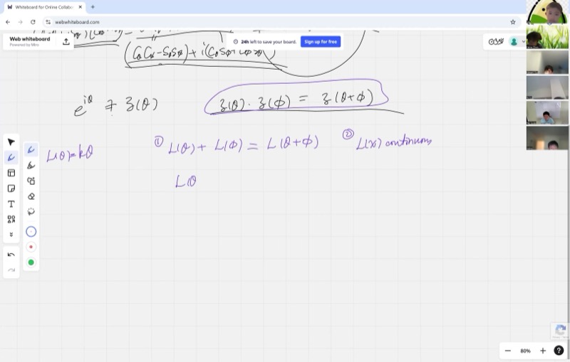
- Multiplicative functions: \(Z(\theta)\cdot Z(\phi) = Z(\theta + \phi)\)
- Connecting multiplicative and additive functions via the logarithm
- Proving \(e^{i\theta} = \cos\theta + i\sin\theta\) (Euler’s formula)
- Logarithm identities: \(\ln(ab) = \ln a + \ln b\)
- Infinitesimal power expansion and identifying the constant \(k = i\)
Lecture Video
Key Frames from the Lecture
Prerequisites
A functional equation is an equation where the unknown is a function rather than a number. Instead of asking “find \(x\) such that \(2x + 3 = 7\),” you ask “find a function \(f\) such that \(f(a + b) = f(a) + f(b)\) for all \(a\) and \(b\).”
The strategy is usually:
- Plug in clever special values (like \(0\), or \(a = b\))
- Build up from integers to rationals to all reals
- Use extra conditions (like continuity) to pin down the answer
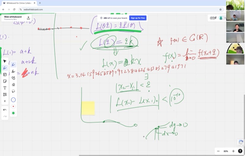
A function \(f(x)\) is continuous if small changes in the input produce small changes in the output – no jumps, no holes, no teleporting.
Formally, \(f\) is continuous at \(x_0\) if:
\[f(x_0) = \lim_{h \to 0} f(x_0 + h)\]
This means: for any desired closeness \(\delta\) in the output, you can find a small enough window \(\epsilon\) around \(x_0\) so that all inputs in that window give outputs within \(\delta\) of \(f(x_0)\).
Graphically, a continuous function can be drawn without lifting the pencil from the paper.
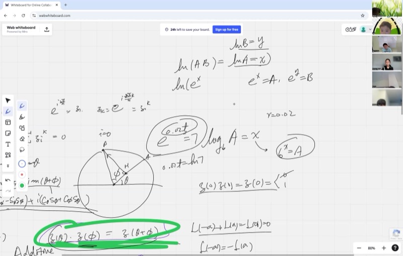
If \(b^x = a\), then \(x = \log_b(a)\). The logarithm answers the question: “what exponent do I put on \(b\) to get \(a\)?”
The natural logarithm \(\ln\) uses base \(e \approx 2.718\):
\[\ln(a) = x \quad \Longleftrightarrow \quad e^x = a\]
Key property: logarithms turn multiplication into addition:
\[\ln(ab) = \ln a + \ln b\]
This is exactly what makes logarithms the bridge between multiplicative and additive functions.
A complex number \(z = x + iy\) can be plotted as the point \((x, y)\) in the plane. If \(|z| = 1\), it lies on the unit circle, and we can write:
\[z = \cos\theta + i\sin\theta\]
where \(\theta\) is the angle from the positive \(x\)-axis. Multiplying two unit complex numbers adds their angles:
\[(\cos\alpha + i\sin\alpha)(\cos\beta + i\sin\beta) = \cos(\alpha + \beta) + i\sin(\alpha + \beta)\]
This multiplication-to-addition connection is the starting point for today’s proof.
From the study of continuously compounded interest and binomial expansion, we showed:
\[e^x = \sum_{n=0}^{\infty} \frac{x^n}{n!} = 1 + x + \frac{x^2}{2!} + \frac{x^3}{3!} + \cdots\]
When \(x\) is very small (infinitesimal), only the first few terms matter:
\[e^x \approx 1 + x \quad \text{(for small } x\text{)}\]
This approximation is the key to finding the constant \(k\) at the end of the proof.
Key Concepts
The Angle-Addition Formula as a Functional Equation
On the unit circle, define \(Z(\theta) = \cos\theta + i\sin\theta\) as the unit complex number at angle \(\theta\). From the cosine and sine addition formulas (proven geometrically by dropping altitudes on the unit circle):
\[\cos(\theta + \phi) = \cos\theta\cos\phi - \sin\theta\sin\phi\] \[\sin(\theta + \phi) = \cos\theta\sin\phi + \sin\theta\cos\phi\]
we can verify that multiplying two unit complex numbers gives:
\[Z(\theta) \cdot Z(\phi) = (\cos\theta + i\sin\theta)(\cos\phi + i\sin\phi) = \cos(\theta+\phi) + i\sin(\theta+\phi) = Z(\theta + \phi)\]
So \(Z\) satisfies the multiplicative functional equation:
When two unit complex numbers are multiplied, their angles add. This means the function \(Z(\theta) = \cos\theta + i\sin\theta\) converts addition of angles into multiplication of numbers — a property that forces \(Z\) to be an exponential.
\[\boxed{Z(\theta) \cdot Z(\phi) = Z(\theta + \phi)}\]
This is the property we will use to prove that \(Z(\theta) = e^{i\theta}\).
Animated visualization – \(e^{i\theta}\) tracing the unit circle as \(\theta\) increases:
Step 1: Additive Functions – \(L(a + b) = L(a) + L(b)\)
Before tackling the multiplicative equation, we prove a foundational result: if a continuous function \(L\) satisfies
\[L(\theta + \phi) = L(\theta) + L(\phi) \quad \text{for all } \theta, \phi \in \mathbb{R}\]
then \(L(\theta) = k\theta\) for some constant \(k\).
Finding \(L(0)\): Set \(\theta = \phi = 0\):
\[L(0) + L(0) = L(0) \implies 2L(0) = L(0) \implies L(0) = 0\]
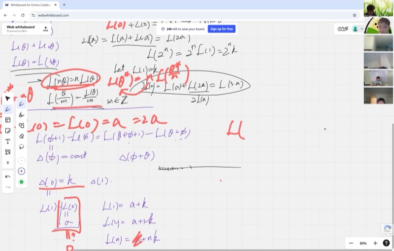
Building up to integers: Set \(\phi = \theta\):
\[L(\theta) + L(\theta) = L(2\theta) \implies L(2\theta) = 2L(\theta)\]
Repeating, \(L(3\theta) = L(2\theta) + L(\theta) = 3L(\theta)\), and by induction:
\[L(n\theta) = nL(\theta) \quad \text{for all positive integers } n\]
Odd function: Set \(\phi = -\theta\):
\[L(\theta) + L(-\theta) = L(0) = 0 \implies L(-\theta) = -L(\theta)\]
So \(L(n\theta) = nL(\theta)\) holds for all integers \(n\) (positive, negative, and zero).
Explore – see that additive continuous functions are lines through the origin:
Drag the slider \(k\) to change the slope. Every continuous additive function is a line through the origin – the only freedom is the slope \(k = L(1)\).
Step 2: Extending to Rational Numbers
We proved \(L(n\theta) = nL(\theta)\) for integer \(n\). Now substitute \(\theta^* = n\theta\), so \(\theta = \theta^*/n\):
\[L(\theta^*) = nL\!\left(\frac{\theta^*}{n}\right) \implies L\!\left(\frac{\theta}{n}\right) = \frac{L(\theta)}{n}\]
Combining both results, for any integers \(n\) and \(m\) (with \(m \neq 0\)):
\[L\!\left(\frac{n}{m}\,\theta\right) = \frac{n}{m}\,L(\theta)\]
Setting \(\theta = 1\) and writing \(q = n/m\):
\[L(q) = qL(1) = kq \quad \text{for every rational number } q\]
Step 3: Using Continuity to Reach All Real Numbers
Rational numbers are dense in the real line: for any real number \(x\), there is a sequence of rationals \(q_1, q_2, q_3, \ldots\) approaching \(x\). For example, the truncated decimal expansions \(3, 3.1, 3.14, 3.141, \ldots\) approach \(\pi\).
Since \(L\) is continuous and \(L(q_n) = kq_n\) for each rational approximation:
\[L(x) = \lim_{n\to\infty} L(q_n) = \lim_{n\to\infty} kq_n = k \cdot \lim_{n\to\infty} q_n = kx\]
\[\boxed{L(\theta) = k\theta \quad \text{for all real } \theta}\]
This is the power of continuity: once you know a function’s values on the rationals, and it has no jumps, you know it everywhere.
Step 4: From Multiplicative to Additive via Logarithm
Now return to the unit complex number \(Z(\theta)\) satisfying \(Z(\theta)\cdot Z(\phi) = Z(\theta + \phi)\).
Define a new function \(f(\theta) = \ln Z(\theta)\). Using the logarithm identity \(\ln(ab) = \ln a + \ln b\):
\[f(\theta) + f(\phi) = \ln Z(\theta) + \ln Z(\phi) = \ln\!\big(Z(\theta) \cdot Z(\phi)\big) = \ln Z(\theta + \phi) = f(\theta + \phi)\]
The logarithm converts the multiplicative equation into an additive one. Since \(Z\) is continuous (it traces a smooth curve on the unit circle) and \(\ln\) is continuous, \(f\) is also continuous. By our theorem from Steps 1–3:
\[f(\theta) = k\theta \implies \ln Z(\theta) = k\theta\]
Exponentiating both sides:
\[\boxed{Z(\theta) = e^{k\theta}}\]
Explore – see \(e^{k\theta}\) for different values of \(k\):
Drag the slider \(k\) to see how the exponential stretches or compresses. The function always passes through \((0, 1)\) because \(Z(0) = e^0 = 1\).
Animated visualization – the functional equation \(f(x+y)=f(x)\cdot f(y)\): why only exponentials work:
Watch how as \(y\) increases, \(f(x+y)\) (purple) always equals the product \(f(x) \cdot f(y)\) (green times red). Only exponential functions have this property.
Set \(\ln a = x\) and \(\ln b = y\). Then \(a = e^x\) and \(b = e^y\), so:
\[ab = e^x \cdot e^y = e^{x+y}\]
Taking logarithms: \(\ln(ab) = x + y = \ln a + \ln b\). The key step is that exponentials convert addition into multiplication — logarithms reverse this correspondence.
Step 5: Finding \(k = i\)
We have established that \(Z(\theta) = e^{k\theta}\) but the constant \(k\) remains to be determined. We use the power series expansion for an infinitesimal angle \(d\theta\):
\[Z(d\theta) = e^{k\,d\theta} = 1 + k\,d\theta + \frac{(k\,d\theta)^2}{2!} + \cdots \approx 1 + k\,d\theta\]
On the unit circle, \(Z(d\theta)\) is the point at a tiny angle \(d\theta\) from \((1, 0)\). Geometrically:
- The real part is \(\cos(d\theta) \approx 1\) (the point barely moves horizontally)
- The imaginary part is \(\sin(d\theta) \approx d\theta\) (the arc length equals the angle in radians)
So \(Z(d\theta) \approx 1 + i\,d\theta\). Comparing with \(1 + k\,d\theta\):
\[k\,d\theta = i\,d\theta \implies k = i\]
Therefore:
This is the culmination of the argument — exponentials, trigonometric functions, and imaginary numbers are unified in a single equation. It states that \(e^{i\theta}\) traces the unit circle, with cosine as the real part and sine as the imaginary part.
\[\boxed{e^{i\theta} = \cos\theta + i\sin\theta}\]
This is Euler’s formula.
Explore – see \(e^{i\theta}\) trace the unit circle:
Drag \(\theta_1\) and watch \(e^{i\theta}\) move around the unit circle. The green segment is \(\cos\theta\) (real part) and the red segment is \(\sin\theta\) (imaginary part).
The Beautiful Consequence: \(e^{i\pi} + 1 = 0\)
Setting \(\theta = \pi\) in Euler’s formula:
\[e^{i\pi} = \cos\pi + i\sin\pi = -1 + 0 = -1\]
Setting \(\theta = \pi\) in Euler’s formula yields one of the most celebrated equations in mathematics — one that relates five fundamental constants using three basic operations.
\[\boxed{e^{i\pi} + 1 = 0}\]
This single equation links five fundamental constants – \(e\), \(i\), \(\pi\), \(1\), and \(0\) – using three basic operations (addition, multiplication, exponentiation). It is often called the most beautiful equation in mathematics.
Cheat Sheet
| Result | Statement |
|---|---|
| Additive functional equation | \(L(\theta + \phi) = L(\theta) + L(\phi)\), continuous \(\implies L(\theta) = k\theta\) |
| Multiplicative functional equation | \(Z(\theta)\cdot Z(\phi) = Z(\theta+\phi)\), continuous \(\implies Z(\theta) = e^{k\theta}\) |
| Euler’s formula | \(e^{i\theta} = \cos\theta + i\sin\theta\) |
| Euler’s identity | \(e^{i\pi} + 1 = 0\) |
| Logarithm converts \(\times\) to \(+\) | \(\ln(ab) = \ln a + \ln b\) |
| Angle addition (cosine) | \(\cos(\theta+\phi) = \cos\theta\cos\phi - \sin\theta\sin\phi\) |
| Angle addition (sine) | \(\sin(\theta+\phi) = \cos\theta\sin\phi + \sin\theta\cos\phi\) |
Proof Strategy Summary
- Start with \(Z(\theta)\cdot Z(\phi) = Z(\theta+\phi)\) (from trig addition formulas)
- Take \(\ln\) of both sides to get additive equation: \(f(\theta) + f(\phi) = f(\theta+\phi)\)
- Prove additive + continuous \(\implies f(\theta) = k\theta\)
- Exponentiate: \(Z(\theta) = e^{k\theta}\)
- Use infinitesimal geometry to find \(k = i\)
The Infinitesimal Argument
\[Z(d\theta) \approx 1 + i\,d\theta \quad \text{(from unit circle geometry)}\]
\[e^{k\,d\theta} \approx 1 + k\,d\theta \quad \text{(from power series)}\]
\[\implies k = i\]