Derivative Techniques Review: Chain Rule, Logarithmic Differentiation & Inverse Function Derivatives
This lesson consolidates the core differentiation techniques needed for the remainder of the course. We review the chain rule, the product and quotient rules, and logarithmic differentiation — a technique that converts complicated products into manageable sums. We also develop the differentiation of inverse functions and examine what occurs when a derivative is unbounded, requiring alternative estimation strategies.
Proficiency with derivative techniques is foundational for the rest of calculus:
- Physics: velocity, acceleration, and force are all obtained by differentiating position — engineers apply the chain rule to complicated motion equations routinely.
- Medicine: drug concentration in the bloodstream follows exponential and rational functions — derivatives determine when a drug is most effective.
- Finance: the rate at which an investment grows depends on derivatives of compound-interest formulas involving products and exponentials.
- Computer graphics: rendering realistic lighting on curved surfaces requires derivatives of composite trigonometric and polynomial functions.
- Climate science: temperature models involve products and compositions of many functions — scientists differentiate them to predict rates of change.
Topics Covered
- Review of the power rule from the binomial expansion: \(\frac{d}{dx} x^r = r\,x^{r-1}\)
- Applying the chain rule to peel apart nested functions layer by layer
- Using the product rule and quotient rule together on complex expressions
- Logarithmic differentiation: turning products into sums via \(\ln\) to simplify derivatives of complicated rational functions
- Derivatives of inverse functions: \(\frac{d}{dx}[f^{-1}(x)] = \frac{1}{f'(f^{-1}(x))}\)
- Estimating \(\operatorname{arccosh}(1.001)\) using differentials and the definition of the derivative
- Recognizing when a derivative is infinite and choosing alternative strategies
Lecture Video
Key Frames from the Lecture
Prerequisites
When one function is inside another — a composite function such as \(f(g(x))\) — the chain rule prescribes how to differentiate:
\[\frac{d}{dx}\bigl[f(g(x))\bigr] = f'(g(x)) \cdot g'(x)\]
One proceeds layer by layer: differentiate the outer function first (leaving the inside unchanged), then multiply by the derivative of the inner function.
Example: If \(h(x) = (3x+1)^5\), then:
\[h'(x) = 5(3x+1)^4 \cdot 3 = 15(3x+1)^4\]
Product rule: When two functions are multiplied together:
\[\frac{d}{dx}[u \cdot v] = u' v + u v'\]
Quotient rule: When one function is divided by another:
\[\frac{d}{dx}\!\left[\frac{u}{v}\right] = \frac{u'v - uv'}{v^2}\]
These rules handle expressions built from simpler components combined by multiplication or division.
The natural logarithm \(\ln(x)\) is the inverse of \(e^x\). It has a key property that makes multiplication simpler:
\[\ln(a \cdot b) = \ln a + \ln b, \qquad \ln\!\left(\frac{a}{b}\right) = \ln a - \ln b, \qquad \ln(a^n) = n\ln a\]
This is why taking \(\ln\) of both sides can convert a complicated product of powers into a clean sum — precisely the technique underlying logarithmic differentiation.
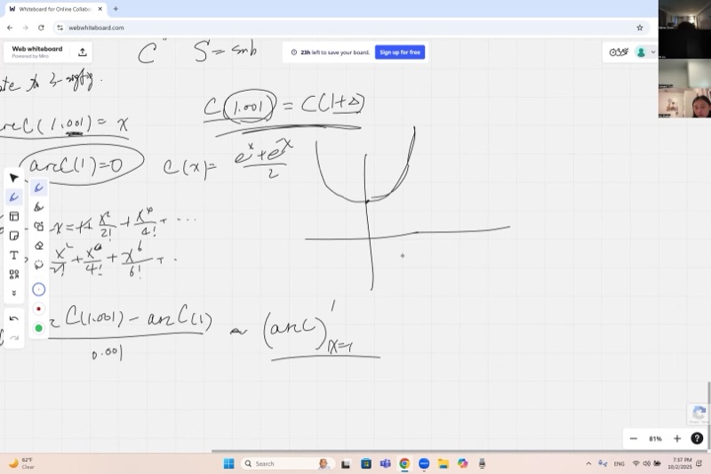
The hyperbolic cosine is defined as:
\[\cosh x = \frac{e^x + e^{-x}}{2}\]
Its graph looks like a U-shaped curve (called a catenary — the shape a hanging chain makes). Key facts:
- \(\cosh 0 = 1\) (the minimum value)
- \(\cosh x\) is an even function: \(\cosh(-x) = \cosh(x)\)
- Its derivative is \(\sinh x = \frac{e^x - e^{-x}}{2}\)
- Its Maclaurin series is \(\cosh x = 1 + \frac{x^2}{2!} + \frac{x^4}{4!} + \cdots\)
Key Concepts
The Power Rule Foundation
Everything starts from the binomial expansion. For any exponent \(r\) (positive, negative, or fractional):
\[(x + dx)^r = x^r\!\left(1 + \frac{dx}{x}\right)^r \approx x^r\!\left(1 + r\,\frac{dx}{x}\right)\]
We retain only the lowest-order infinitesimal. Subtracting \(x^r\) and dividing by \(dx\):
\[\frac{d}{dx}\,x^r = r\,x^{r-1}\]
This extends beyond simple powers — via power (Maclaurin) expansions, it handles polynomials, rational functions, exponentials (\(e^x = \sum x^k/k!\)), and trig functions.
Chain Rule in Action: Peeling Layers
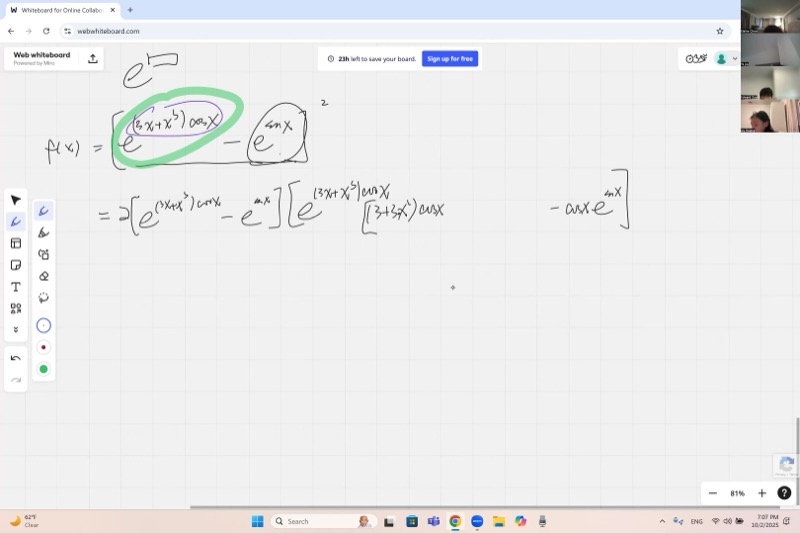
Consider the function from class:
\[f(x) = \Bigl(e^{3x + x^3\cos x} - e^{\sin x}\Bigr)^2\]
To differentiate, work outside-in:
Layer 1 — the square: The outermost operation is \((\cdots)^2\). By the power rule:
\[f'(x) = 2\Bigl(e^{3x + x^3\cos x} - e^{\sin x}\Bigr) \cdot \frac{d}{dx}\Bigl(e^{3x + x^3\cos x} - e^{\sin x}\Bigr)\]
Layer 2 — the exponentials: Differentiate each term inside the bracket separately.
For \(e^{\sin x}\): the derivative of \(e^u\) is \(e^u \cdot u'\), so:
\[\frac{d}{dx}\,e^{\sin x} = e^{\sin x}\cdot \cos x\]
For \(e^{3x + x^3\cos x}\): same pattern, but the inner function is more complex:
\[\frac{d}{dx}\,e^{3x + x^3\cos x} = e^{3x + x^3\cos x}\cdot \frac{d}{dx}(3x + x^3\cos x)\]
Layer 3 — the inner function: Apply the product rule to \(x^3 \cos x\):
\[\frac{d}{dx}(3x + x^3\cos x) = 3 + 3x^2\cos x - x^3\sin x\]
Assembling all components yields the complete derivative — lengthy, but each step is mechanical.
Animated visualization – chain rule unwinding: peeling nested functions layer by layer:
Explore how the chain rule works on nested functions:
Logarithmic Differentiation
When a function is a large product and quotient of powers, direct application of the product rule is unwieldy. Instead, one takes \(\ln\) of both sides.
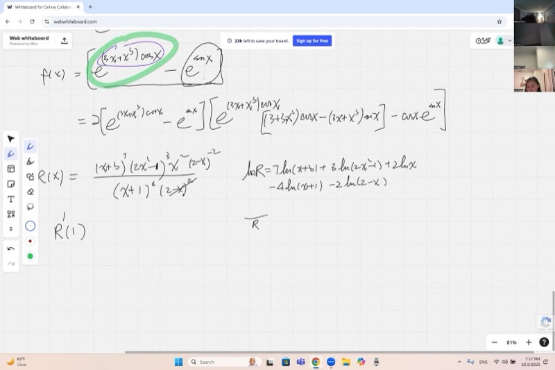
Example from class: Find \(R'(1)\) where
\[R(x) = \frac{(x+3)^7 \cdot (2x^2-1)^3 \cdot x^2}{(x+1)^4 \cdot (2-x)^2}\]
Step 1 — Take \(\ln\) of both sides:
\[\ln R = 7\ln(x+3) + 3\ln(2x^2-1) + 2\ln x - 4\ln(x+1) - 2\ln(2-x)\]
Products become sums, quotients become differences, and exponents become coefficients.
Step 2 — Differentiate both sides:
\[\frac{R'}{R} = \frac{7}{x+3} + \frac{12x}{2x^2-1} + \frac{2}{x} - \frac{4}{x+1} + \frac{2}{2-x}\]
On the left, the chain rule gives \(\frac{1}{R}\cdot R'\). On the right, each logarithmic term differentiates cleanly. Note the last term carefully: the derivative of \((2-x)\) is \(-1\), so the two negatives combine to give \(+\frac{2}{2-x}\).
Step 3 — Solve for \(R'\):
When a function is a large product and quotient of powers, take \(\ln\) of both sides first. This converts products into sums, simplifying differentiation. Then solve for \(R'\) by multiplying both sides by \(R\).
\[R'(x) = R(x)\left[\frac{7}{x+3} + \frac{12x}{2x^2-1} + \frac{2}{x} - \frac{4}{x+1} + \frac{2}{2-x}\right]\]
To evaluate at \(x = 1\): compute \(R(1)\) once, then substitute \(x=1\) into each simple fraction and sum. This is far more efficient than expanding the product rule across five factors.
Animated visualization – logarithmic differentiation: transforming a product into a sum of logs step by step:
Logarithmic differentiation exploits the logarithm laws to decompose a product into a sum. Differentiating a sum is straightforward — one differentiates term by term. The result is equivalent to the product rule, but organized so that each factor contributes one clean fraction.
Each term such as \(\frac{7}{x+3}\) arises from “holding every other factor fixed, differentiating only \((x+3)^7\), and dividing by the whole \(R\).” This is precisely what the generalized product rule produces.
Visualize the function \(R(x)\) and its derivative:
Derivatives of Inverse Functions
If \(y = f(x)\) has an inverse \(x = f^{-1}(y)\), then:
To differentiate an inverse function, take the reciprocal of the derivative of the original function. If \(f'\) is known, then the derivative of \(f^{-1}\) equals \(1/f'\) evaluated at the corresponding point.
\[\frac{d}{dy}\bigl[f^{-1}(y)\bigr] = \frac{1}{f'(x)} = \frac{1}{f'\!\bigl(f^{-1}(y)\bigr)}\]
Graphically, the derivative of the inverse at a point is the reciprocal of the derivative of the original function at the corresponding point. If \((x_0, y_0)\) is on the graph of \(f\), then \((y_0, x_0)\) is on the graph of \(f^{-1}\), and:
\[\bigl(f^{-1}\bigr)'(y_0) = \frac{1}{f'(x_0)}\]
Explore \(\cosh x\) and \(\operatorname{arccosh} x\) as reflections across \(y = x\):
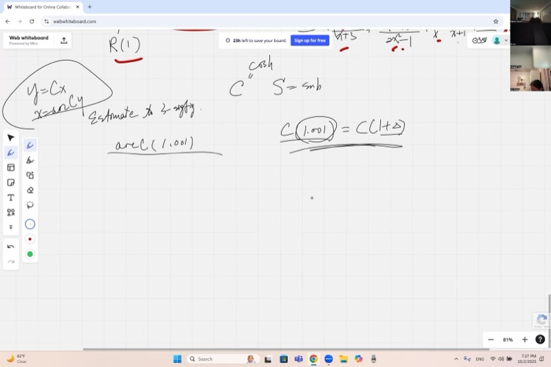
Estimating \(\operatorname{arccosh}(1.001)\): When Derivatives Blow Up
We seek to estimate \(\operatorname{arccosh}(1.001)\) to three significant figures.
First attempt — using the derivative:
Since \(\operatorname{arccosh}(1) = 0\) (because \(\cosh(0) = 1\)), and \(1.001\) is close to \(1\), one might attempt:
\[\operatorname{arccosh}(1.001) \approx \operatorname{arccosh}(1) + 0.001 \cdot \frac{d}{dy}\operatorname{arccosh}(y)\Big|_{y=1}\]
However, the derivative of \(\operatorname{arccosh}\) at \(y=1\) is \(\frac{1}{\sinh(\operatorname{arccosh}(1))} = \frac{1}{\sinh(0)} = \frac{1}{0} = \infty\).
Graphically, \(\cosh x\) has a horizontal tangent at \(x = 0\), so its inverse \(\operatorname{arccosh}\) has a vertical tangent at \(y = 1\). The linear approximation fails completely.
Consequence: The value \(\operatorname{arccosh}(1.001)\) is much larger than \(0.001\) would suggest — it grows as a fractional power of the increment, not linearly.
Second attempt — solve directly from the definition:
Set \(\cosh x = 1.001\), i.e., \(\frac{e^x + e^{-x}}{2} = 1.001\). Let \(u = e^x\):
\[u + \frac{1}{u} = 2.002 \quad \Longrightarrow \quad u^2 - 2.002\,u + 1 = 0\]
By the quadratic formula:
\[u = \frac{2.002 \pm \sqrt{2.002^2 - 4}}{2} = 1.001 \pm \sqrt{1.001^2 - 1}\]
Since \(x > 0\), we pick the \(+\) sign:
\[e^x = 1.001 + \sqrt{0.002001}\]
Now \(\sqrt{0.002001} \approx 0.04473\), so \(e^x \approx 1.04573\), and:
\[x = \ln(1.04573) \approx 0.04473 - \frac{0.04473^2}{2} + \cdots \approx 0.0447\]
The answer \(\operatorname{arccosh}(1.001) \approx 0.0447\) is far larger than \(0.001\) — confirming that the linear derivative approach could not work here.
Whenever one estimates \(f(a + \epsilon)\) using the linear approximation \(f(a + \epsilon) \approx f(a) + \epsilon\,f'(a)\), this requires \(f'(a)\) to be finite. If the derivative is unbounded, the function changes by a fractional power of \(\epsilon\) rather than linearly, and an alternative strategy is needed — such as solving the defining equation directly.
Cube Roots Near Zero: Another Infinite-Derivative Trap
The same issue arises with \(\sqrt[3]{0.007}\). If one attempts to expand \(x^{1/3}\) around \(x = 0\):
\[\frac{d}{dx}\,x^{1/3} = \frac{1}{3}\,x^{-2/3}\]
At \(x = 0\), this is \(\infty\). The tangent line at the origin is vertical, so a Taylor expansion at that point does not exist. Instead, one expands around a nearby convenient point (such as \(x = 0.008 = 0.2^3\)) where the derivative is finite.
See the vertical tangent of \(y = x^{1/3}\) at the origin:
Cheat Sheet
| Formula | Notes |
|---|---|
| \(\frac{d}{dx}\,x^r = r\,x^{r-1}\) | Power rule — works for any real \(r\) |
| \(\frac{d}{dx}\,e^{u} = e^{u}\cdot u'\) | Exponential + chain rule |
| \(\frac{d}{dx}[f(g(x))] = f'(g(x))\cdot g'(x)\) | Chain rule — peel layers outside-in |
| \((uv)' = u'v + uv'\) | Product rule |
| \(\left(\frac{u}{v}\right)' = \frac{u'v - uv'}{v^2}\) | Quotient rule |
Logarithmic Differentiation
For \(R(x) = \prod f_i(x)^{a_i}\), take \(\ln\) of both sides:
\[\ln R = \sum a_i \ln f_i(x) \qquad \Longrightarrow \qquad \frac{R'}{R} = \sum \frac{a_i\,f_i'(x)}{f_i(x)}\]
\[R'(x) = R(x)\sum \frac{a_i\,f_i'(x)}{f_i(x)}\]
Inverse Function Derivative
\[\frac{d}{dy}\bigl[f^{-1}(y)\bigr] = \frac{1}{f'\!\bigl(f^{-1}(y)\bigr)}\]
Hyperbolic Functions
\[\cosh x = \frac{e^x + e^{-x}}{2}, \qquad \sinh x = \frac{e^x - e^{-x}}{2}\]
\[\frac{d}{dx}\cosh x = \sinh x, \qquad \frac{d}{dx}\sinh x = \cosh x\]
\[\operatorname{arccosh}(y) = \ln\!\left(y + \sqrt{y^2 - 1}\right), \quad y \ge 1\]