Propagated Error and Logarithmic Differentiation for Percent Error Analysis
Every measurement carries inherent error – a ruler has finite precision, a scale introduces rounding, and so forth. When these measurements are substituted into a formula, the errors propagate through the calculation. This lesson develops the theory of error propagation, introduces the logarithmic differentiation technique for simplifying the analysis, and explains why independent errors combine via a Pythagorean (root-sum-of-squares) rule rather than by direct addition. The result is a systematic method for assessing the reliability of any calculated quantity.
Every measurement in practice carries some inaccuracy. When these measurements enter a formula, the errors propagate into the result. Understanding this process is essential:
- Aerospace engineering: engineers calculate how small errors in thrust, fuel mass, and timing compound into trajectory deviations – inaccurate estimates can cause a spacecraft to miss its target by a large margin
- Medical diagnostics: a blood test result depends on instrument precision, sample volume, and chemical concentrations – physicians must assess the reliability of the result before making a diagnosis
- Structural engineering: if every beam length has a small measurement error, the total height uncertainty of a structure depends on how those errors combine – engineers must ensure the building meets specifications
- Measurement systems: when tracking an object’s speed using radar, errors in distance and time measurements propagate into the velocity calculation – one must determine whether the computed speed is reliable
- Industrial processes: scaling up a process means small errors in each measured quantity accumulate – percent error analysis determines whether the output remains within acceptable tolerances
Topics Covered
- Propagated error in multi-variable formulas: \(\Delta F\) from \(\Delta G\), \(\Delta M\), \(\Delta m\), \(\Delta r\)
- Logarithmic differentiation to simplify percent error calculations
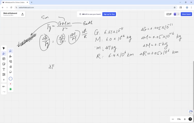
- Newton’s Law of Gravitation: \(F_G = \frac{G M m}{r^2}\)
- Percent error vs. absolute error: \(\frac{dF}{F}\) vs. \(dF\)
- Pythagorean (Gaussian) sum for independent errors: \(\sqrt{\left(\frac{\Delta a}{a}\right)^2 + \left(\frac{\Delta b}{b}\right)^2 + \cdots}\)
- Comparing measurement strategies: repeated measurements and averaging
Lecture Video
Key Frames from the Lecture
Prerequisites
Every object with mass attracts every other object with mass. The gravitational force between them is:
\[F_G = \frac{G \cdot M \cdot m}{r^2}\]
where:
- \(G \approx 6.67 \times 10^{-11} \; \text{N m}^2/\text{kg}^2\) is the universal gravitational constant
- \(M\) and \(m\) are the masses of the two objects (e.g., the Earth and a person)
- \(r\) is the distance between their centers
This formula gives the weight of an object: the gravitational force the Earth exerts on it.
When a number is written as \(6.67 \times 10^{-11}\), it has three significant figures. The true value could be anywhere from \(6.665 \times 10^{-11}\) to \(6.675 \times 10^{-11}\).
The rounding error (or uncertainty) is half the last digit’s place value:
\[\Delta = \frac{1}{2} \times 10^{\text{place of last digit}}\]
For \(6.67 \times 10^{-11}\), the last digit is in the hundredths place of the coefficient, so \(\Delta = 0.005 \times 10^{-11}\).
The number of significant figures in your least precise measurement limits the precision of your final answer.
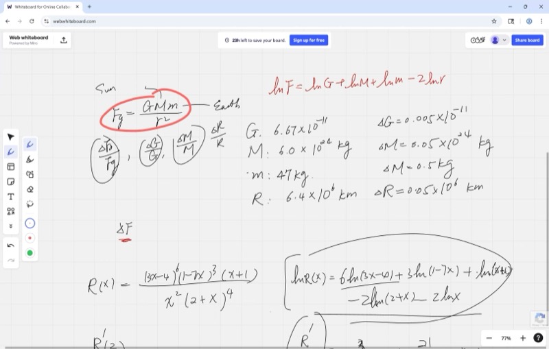
When a function is a product or quotient of many factors, taking the natural log first converts the expression into sums and differences, which are much simpler to differentiate.
For example, if \(R(x) = \frac{(3x-4)^6 (1-7x)^3 (x+1)}{x^2 (2+x)^4}\), then:
\[\ln R(x) = 6\ln(3x-4) + 3\ln(1-7x) + \ln(x+1) - 2\ln(x) - 4\ln(2+x)\]
Each term then differentiates readily using the chain rule, yielding:
\[\frac{R'(x)}{R(x)} = \frac{18}{3x-4} - \frac{21}{1-7x} + \frac{1}{x+1} - \frac{2}{x} - \frac{4}{2+x}\]
This avoids the complexity of applying the quotient rule and product rule to the original expression.
The differential \(df\) represents a tiny change in \(f\) caused by a tiny change \(dx\) in the input:
\[df = f'(x) \cdot dx\]
In error analysis, we reinterpret \(dx\) as the measurement error \(\Delta x\). Then \(df \approx \Delta f\) gives us the propagated error – how much the output changes due to input uncertainty.
The percent error (or relative error) is:
\[\frac{df}{f} = \frac{\Delta f}{f}\]
This tells you what fraction of the value is uncertain, which is often more meaningful than the absolute error alone.
The Pythagorean theorem says that for a right triangle with legs \(a\) and \(b\) and hypotenuse \(c\):
\[c = \sqrt{a^2 + b^2}\]
In error analysis, we use a Pythagorean sum of percent errors because independent errors are unlikely to all push in the same direction. They behave like perpendicular (orthogonal) components, so the total error magnitude is the square root of the sum of squares – just like finding the hypotenuse.
Key Concepts
Setting Up the Gravitational Force Problem
We want to calculate the gravitational force on a person standing on Earth’s surface using measured values. Each measurement carries a rounding error:
| Quantity | Value | Error (\(\Delta\)) |
|---|---|---|
| \(G\) (gravitational constant) | \(6.67 \times 10^{-11}\) | \(0.005 \times 10^{-11}\) |
| \(M\) (mass of Earth) | \(5.97 \times 10^{24}\) kg | \(0.005 \times 10^{24}\) kg |
| \(m\) (mass of person) | \(47\) kg | \(0.5\) kg |
| \(r\) (radius of Earth) | \(6.4 \times 10^{6}\) m | \(0.05 \times 10^{6}\) m |
The force is:
\[F_G = \frac{G \cdot M \cdot m}{r^2}\]
The problem: find \(\Delta F_G\), the propagated error in the calculated force.
Why Direct Differentiation is Impractical
Attempting to compute \(\Delta F_G\) directly by differentiating \(F_G\) with respect to each variable and applying the quotient rule leads to a cumbersome calculation involving four variables in products and quotients. The algebra is tedious and error-prone.
The remedy: use logarithmic differentiation to convert to percent errors.
The Logarithmic Differentiation Shortcut
Take the natural log of both sides of the force equation:
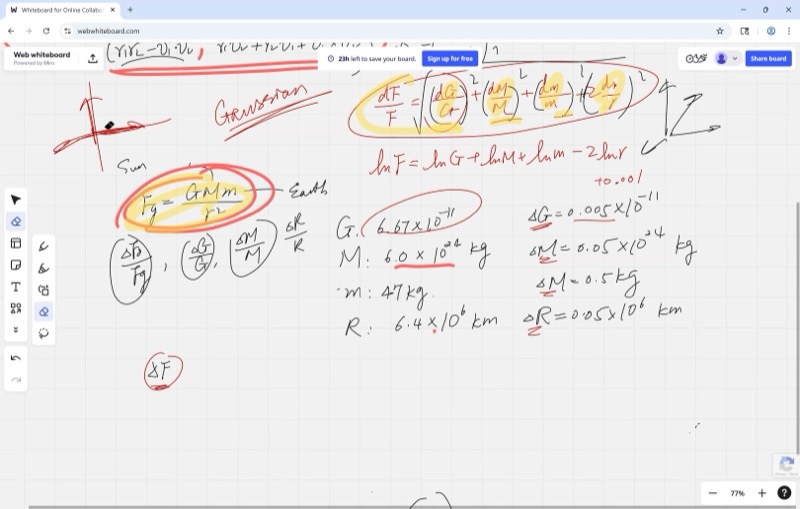
\[\ln F_G = \ln G + \ln M + \ln m - 2\ln r\]
The product and quotient have become a simple sum. Differentiating:
When a formula is built from quantities multiplied and divided together, taking the natural log converts everything into addition and subtraction. That makes it simple to see how each measurement’s percent error feeds into the final answer.
\[\frac{dF_G}{F_G} = \frac{dG}{G} + \frac{dM}{M} + \frac{dm}{m} - 2\,\frac{dr}{r}\]
Each term on the right is a percent error – the ratio of the uncertainty to the value itself. This is far more informative than computing absolute errors, because a small absolute error in \(G\) (of order \(10^{-11}\)) does not indicate high accuracy; one must compare it to \(G\) itself.
Interactive demonstration – percent error in radius and its effect on force:
Drag \(a\) to change the radius. The red dashed tangent line shows the linear approximation – its slope is \(-2/a^3\), reflecting the factor of \(2\) in front of \(\frac{dr}{r}\). A small change in \(r\) causes roughly twice as large a percent change in \(F\).
Interactive: Absolute vs. Relative Error Comparison
Percent Error Visualization: Absolute vs. Relative Error
Use the sliders (or press Play) to vary the error multipliers for \(G\) and \(m\). The blue bars show percent errors \(\frac{\Delta x}{x}\), the red bars show (scaled) absolute errors, and the total Pythagorean percent error is displayed at top right. Notice how the least precise measurements dominate the total.
Computing Each Percent Error
Now we plug in the numbers:
\[\frac{\Delta G}{G} = \frac{0.005}{6.67} \approx 0.00075 \approx 0.075\%\]
\[\frac{\Delta M}{M} = \frac{0.005}{5.97} \approx 0.00084 \approx 0.084\%\]
\[\frac{\Delta m}{m} = \frac{0.5}{47} \approx 0.0106 \approx 1.06\%\]
\[2 \cdot \frac{\Delta r}{r} = 2 \cdot \frac{0.05}{6.4} \approx 0.0156 \approx 1.56\%\]
Observe that the first two terms (around \(0.1\%\)) are small compared to the last two (around \(1\%\)). Dropping the first two would barely change the final answer – the least precise measurement dominates the analysis.
The Pythagorean Sum: Why We Don’t Just Add
If we simply added all four percent errors, we would get the worst-case upper bound – as if every error happened to push in the same direction. But in reality, errors are independent (Gaussian): one measurement might read too high while another reads too low.
Independent errors are like perpendicular axes – a deviation in \(G\) doesn’t affect the deviation in \(m\). So the proper way to combine them is the Pythagorean sum (also called the root-sum-of-squares):
Because independent measurement errors are unlikely to all push in the same direction, we combine them like the legs of a right triangle rather than simply adding them up. The total percent error is always smaller than the worst-case sum.
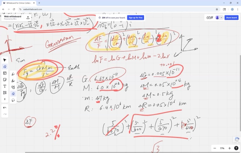
\[\frac{\Delta F_G}{F_G} = \sqrt{\left(\frac{\Delta G}{G}\right)^2 + \left(\frac{\Delta M}{M}\right)^2 + \left(\frac{\Delta m}{m}\right)^2 + \left(2\frac{\Delta r}{r}\right)^2}\]
Interactive demonstration – Pythagorean sum versus simple sum of two errors:
Drag \(a\) and \(b\) to represent two error magnitudes. The green and orange segments are the “legs” (individual errors), the purple dashed line is the Pythagorean hypotenuse (realistic combined error), and the red dot shows the simple sum (worst case). The Pythagorean sum is always smaller or equal.
Interactive: Log Differentiation Decomposition
Log Differentiation: d(ln F) Decomposition
Press “Animate Steps” or drag the step slider to walk through the log differentiation process: from the original product formula, through taking ln, differentiating, interpreting as percent errors, and finally combining them via the Pythagorean sum.
Crunching the Numbers
Plugging in and including all four terms:
\[\frac{\Delta F_G}{F_G} = \sqrt{(0.00075)^2 + (0.00084)^2 + (0.0106)^2 + (0.0156)^2}\]
\[= \sqrt{0.0000006 + 0.0000007 + 0.000112 + 0.000243}\]
\[= \sqrt{0.000356} \approx 0.0189 \approx 2.1\%\]
Notice that the first two terms contribute almost nothing under the square root – as expected, the least precise measurements dominate.
From Percent Error Back to Absolute Error
The percent error \(\frac{\Delta F_G}{F_G}\) is not the final answer. We still need to find \(\Delta F_G\) itself. First, compute \(F_G\) from the original formula:
\[F_G = \frac{(6.67 \times 10^{-11})(5.97 \times 10^{24})(47)}{(6.4 \times 10^{6})^2} \approx 459 \;\text{N}\]
This is close to \(47 \times 9.8 = 460.6\) N – a good sanity check, since \(g \approx 9.8 \;\text{m/s}^2\).
Then the absolute error is:
\[\Delta F_G = F_G \times \frac{\Delta F_G}{F_G} \approx 459 \times 0.021 \approx 10 \;\text{N}\]
That is roughly 2 pounds of uncertainty in the calculated weight – a reasonable result.
Comparing Measurement Strategies
Suppose you want to measure a length and have two rulers:
| Ruler | Smallest marking | Error \(\Delta L\) |
|---|---|---|
| Ruler 1 (meter stick) | 1 cm | 0.5 cm |
| Ruler 2 (fine ruler) | 1 mm | 0.1 cm |
Three strategies:
- A: Use Ruler 1 five times, take the average
- B: Use Ruler 2 once
- C: Combine A’s and B’s data optimally
For strategy A, each measurement \(x_1, x_2, \ldots, x_5\) is independent with error \(\Delta L = 0.5\) cm. The average is:
\[\bar{x} = \frac{x_1 + x_2 + x_3 + x_4 + x_5}{5}\]
Since the errors are independent, the Pythagorean sum applies to the numerator, and dividing by 5 gives:
\[\Delta \bar{x} = \frac{\sqrt{5 \cdot (0.5)^2}}{5} = \frac{0.5}{\sqrt{5}} \approx 0.22 \;\text{cm}\]
If you repeat a measurement \(n\) times and take the average, the error shrinks by a factor of \(\frac{1}{\sqrt{n}}\). Four measurements cut the error in half; to cut it by a factor of ten, you need one hundred measurements.
\[\Delta \bar{x} = \frac{\Delta x}{\sqrt{n}}\]
Repeated independent measurements improve accuracy by a factor of \(\frac{1}{\sqrt{n}}\), where \(n\) is the number of measurements.
Strategy B gives \(\Delta L = 0.1\) cm in a single measurement – better than A’s \(0.22\) cm!
Strategy C (combining data from both) can do even better by weighting each measurement by its precision – a topic for future study.
Cheat Sheet
| Formula | What it means |
|---|---|
| \(F_G = \dfrac{GMm}{r^2}\) | Newton’s Law of Gravitation |
| \(\ln F_G = \ln G + \ln M + \ln m - 2\ln r\) | Log trick: products become sums |
| \(\dfrac{dF}{F} = \dfrac{dG}{G} + \dfrac{dM}{M} + \dfrac{dm}{m} - 2\dfrac{dr}{r}\) | Percent errors from log differentiation |
| \(\dfrac{\Delta F}{F} = \sqrt{\sum_i \left(\frac{\Delta x_i}{x_i}\right)^2}\) | Pythagorean sum for independent errors |
| \(\Delta \bar{x} = \dfrac{\Delta x}{\sqrt{n}}\) | Error reduction by averaging \(n\) measurements |
Key Principles
- Percent error > absolute error: always compare \(\frac{\Delta x}{x}\), not \(\Delta x\) alone
- Log differentiation: when variables are multiplied/divided, take \(\ln\) first to simplify
- Pythagorean sum: independent errors combine as \(\sqrt{a^2 + b^2}\), not \(a + b\)
- Weakest link: your answer’s precision is limited by the least precise measurement
- Don’t forget the last step: \(\Delta F = F \times \frac{\Delta F}{F}\) – always convert back to absolute error